Today, we’re going to dive into the world of reinforcement learning (RL) and explore one of the fields most dominant algorithms, Proximal Policy Optimization. PPO is hands-down one of the most popular RL algorithm out there, and for good reason! Its winning combo of simplicity, efficiency, and stability has made it a go-to choice for a wide range of applications, from robotics to gaming and most recently, teaching Large Language Models like ChatGPT to be seem more human!

By the end, you’ll have a solid understanding of the principles behind PPO, enabling you to utilize this powerful RL tool in your own projects. So, without further ado, let’s dive into the world of Proximal Policy Optimization.

Overview

Imagine you’re learning to drive a car. You’re super excited to get out onto the road, but cars can be dangerous and you are more than a little nervous of damaging the car or even hurting someone. If you accelerate or turn too quickly you could easily lose control of the car. On the other hand, if you slowly increase how fast you are driving you will consistently build up the skills and confidence to handle more challenging situations allowing you to quickly go from the car park to the motorways!

The Proximal Policy Optimization (PPO) algorithm works in a similar way. It helps a machine learning agent learn how to make the right decisions by taking small steps towards better actions, rather than making large, unpredictable jumps. This helps to ensure that the agent doesn’t “lose control of the car” and end up making bad decisions that are difficult to recover from.

PPO achieves this by measuring how much the agent’s policy has changed compared to the previous one and clipping this change within a certain range. This is like constraining the size of each step taken by the agent so that it doesn’t deviate too far from the previous policy.

PPO Components

Actor Critic Architecture

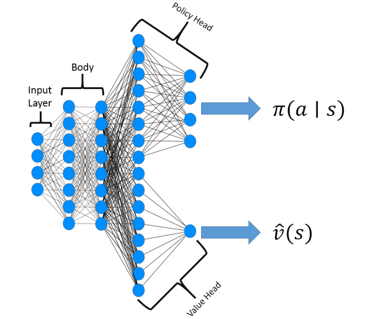
PPO commonly utilises the Actor-Critic architecture, which consists of two neural networks: the Actor network and the Critic network.

Actor \(\pi(a|s)\): network responsible for learning the policy (i.e., deciding which actions to take). This outputs a probability distribution over possible actions. The Actor’s parameters are adjusted using gradient descent based on the feedback provided by the Critic.

Critic \(\hat{v}(s)\): network estimates the value function (i.e., evaluating how good it is to be in a given state). The value function represents the expected cumulative rewards from a given state, following the current policy. The Critic is usually another neural network that takes the state as input and predicts the state’s value.

The Actor-Critic method helps reduce the variance in gradient estimation, a common issue in Policy Gradient methods. It does so by utilising the Critic’s value estimates to compute the “advantage” for each action taken, which represents how much better an action is compared to the average action in a given state, according to the Critic’s estimation.

By using the advantage, the Actor’s policy is updated to prefer actions with higher advantages, effectively balancing exploration and exploitation for more stable learning. However, the Critic’s value estimates introduce some bias into the learning process, as they are approximations and might not be entirely accurate. This bias can affect the learning process, potentially causing the agent to converge to a sub-optimal policy.

Objective Function

PPO’s objective function encourages the agent to take actions that lead to higher rewards. It computes the probability ratio of the new policy (from the Actor network) to the old policy for each action taken, multiplied by the advantage estimate based on the Critic networks value function. PPO calculates this advantage using the Generalised Advantage Estimation algorithm.

Clipped Objective Function

PPO introduces a clipped objective function to prevent large policy updates. This clipping helps to ensure that the agent can make steady progress towards achieving its goals without getting stuck or falling off track. If the probability ratio is between (1-epsilon) and (1+epsilon), it remains unchanged. If it’s outside this range, the clipped ratio is used instead, preventing updates from becoming too large. This clipped function ensures that the new policy doesn’t stray too far from the old one, leading to more stable learning.

Policy Gradient Objective:

\[L^{PG}(\theta )= E_{t}[log_{\pi\theta}(a_t|s_t) * A_t]\]

PPO Clipped Objective:

\[L^{CLIP}(\theta) = \hat{E}_t[ min(r_t(\theta)\hat{A}_t, clip(r_t(\theta), 1-\varepsilon, 1 + \varepsilon) * \hat{A}_t)]\]

The equation above represents the clipped surrogate loss function, \(L^{CLIP}(\theta)\), used in PPO. Let’s break down the expression:

1. \(L^{CLIP}(\theta)\) denotes the clipped surrogate loss function that depends on the policy parameters, \(\theta\). We use this function to update our PPO policy in the right direction.

2. The symbol \(\hat{E}_t\) means we’re taking an average over time, considering different moments when the agent makes decisions. This is refereed to as taking the expectation over time steps t.

3. \(r_t(θ)\) represents how different the new policy is compared to the old one. It’s a ratio that tells us how likely the agent is to take a certain action under the new policy compared to the old policy. This ratio is defined as \(\frac{\pi_{\theta}(a_t \vert s_t)}{\pi_{\theta_{old}}(a_t \vert s_t)}\) , where \(\pi_{\theta}(a_t \vert s_t)\) denotes the probability of taking action \(a_t\) given state \(s_t\) under the policy with parameters \(\theta\) at the time step \(t\). Notice that this ratio replaces the log probability in the original Policy Gradient Objective.

4. \(\hat{A}_t\) measures how good an action is compared to the average action at a specific situation (state). A higher value means the action is expected to yield a better outcome. This estimation is known as the ‘advantage’.

5. \(clip(r_t(\theta), 1-\varepsilon, 1 + \varepsilon)\) is a clipping function that limits the value of \(r_t(θ)\) to the range \([1 - ε, 1 + ε]\), where \(ε\) is a small positive constant. This way, the loss function balances between improving the policy and keeping it stable.

6. \(min(...)\)takes the smallest value between two expressions: one without the clipping function and one with it. This way, the loss function balances between improving the policy and keeping it stable.

Generalised Advantage Estimate

To understand GAE, let’s first introduce the concept of “advantage.” Advantage is the difference between the actual value of a state-action pair and the estimated value of a state. In simpler terms, advantage tells us how much better an action is compared to the average action in a given state.

GAE uses aspects of both Temporal Difference (TD) and Monte Carlo (MC) methods:

1. GAE uses Temporal Difference Error to calculate a series of n-step returns, which are weighted sums of rewards and value function estimates over n steps into the future. These n-step returns help us understand the short-term consequences of our actions.
2. GAE then combines these n-step returns using a weighting factor lambda (λ), which ranges from 0 to 1. When λ is close to 0, GAE relies more on short-term returns (like Temporal Difference Error). When λ is close to 1, GAE relies more on long-term returns (like Monte Carlo Estimation).
3. Finally, GAE calculates the weighted sum of these n-step returns to create a “generalised” advantage estimate. This estimate balances short-term and long-term consequences, offering a more robust way to update the value function.

Generalised Advantage Estimation combines the strengths of Monte Carlo Estimation and Temporal Difference Error by using n-step returns and a weighting factor λ. By adjusting λ, GAE can balance the focus on short-term and long-term consequences, resulting in a more effective and flexible approach for estimating the value function in Policy Gradient algorithms.

Update Epochs

To ensure that the agent’s policy updates are conservative, PPO performs multiple epochs of weight updates on its trainable parameters based on the same training data. This allows PPO to be more sample-efficient than other policy gradient methods. PPO processes data in mini-batches and epochs. After collecting a set of trajectories (sequences of states, actions, and rewards), it divides them into smaller mini-batches. Then, it performs multiple gradient updates for each mini-batch, iterating over the entire dataset for a fixed number of epochs. We do this for several reasons.

1. Improved Stability: Using mini-batches is a form of stochastic gradient descent, which has been shown to have better convergence properties compared to batch gradient descent. It helps escape local minima and find better solutions in the optimisation landscape.
2. Improved Convergence: Running multiple optimisation epochs with mini-batches tends to result in better convergence and stability of the learning process.
3. Improved Efficiency: allows the model to learn more effectively by updating its parameters multiple times based on different subsets of the same data.

Conclusion

Throughout this blog post, we delved into the inner workings of the Proximal Policy Optimisation (PPO) algorithm and its various components, such as the Actor-Critic architecture, the clipped objective function, Generalised Advantage Estimation, and the use of mini-batches and update epochs. These elements come together to create a powerful reinforcement learning algorithm that provides controlled policy updates and stable learning.

PPO’s effectiveness in a wide range of applications showcases its versatility and robustness, making it a valuable tool for reinforcement learning enthusiasts and practitioners. As you embark on your journey in reinforcement learning, consider incorporating PPO into your toolkit to tackle complex problems and drive innovation in AI. The knowledge you’ve gained here will serve as a strong foundation for your future projects and help you unlock the full potential of reinforcement learning. Keep learning and experimenting!

Resources

Here are some more resources to help you learn more about PPO.

Proximal Policy Optimization Algorithms: https://arxiv.org/abs/1707.06347

High-Dimensional Continuous Control Using Generalized Advantage Estimation: https://arxiv.org/abs/1506.02438.pdf

Hugging Face RL Course: Unit 8 Clipped Surrogate Objective: https://huggingface.co/deep-rl-course/unit8/clipped-surrogate-objective?fw=pt

CleanRL: https://github.com/vwxyzjn/cleanrl